
Suppose you worked in industry, and your boss calls you to his office and says they want to enter the emerging "iThingy" market. He wants to offer customized iThingies, and it's important to have an algorithm that, given a specification, can efficiently construct a design that meets the maximum number of requirements in the lowest cost way.

You try for weeks but just can't seem to find an efficient solution. Every solution that you come up with amounts to trying all combinations of components, in exponential time. More efficient algorithms fail to find optimal solutions.
You don't want to have to go your boss and say "I'm sorry I can't find an efficient solution. I guess I'm just too dumb."

You would like to be able to confidently stride into his office and say "I can't find an efficient solution because no such solution exists!" Unfortunately, proving that the problem is inherently intractable is also very hard: in fact, no one has succeeded in doing so.
Today we introduce a class of problems that no one has been able to prove is intractable, but nor has anyone been able to find an efficient solution to any of them.

If you can show that the iThingy configuration problem is one of these problems, you can go to your boss and say, "I can't find an efficient solution, but neither can all these smart and famous computer scientists!"
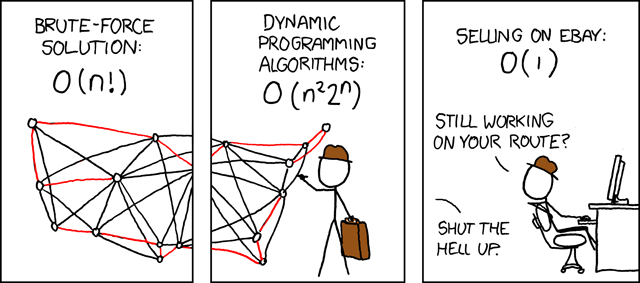
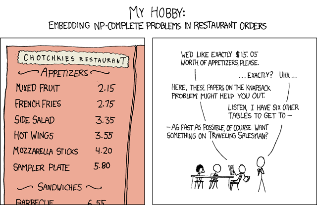
(In Topic 25 we'll cover what you would say next. Thanks to Garey & Johnson (1979) for the story & images.)
For most of this semester, we abstracted away from the study of particular implementations to study the computational complexity of algorithms independently of their implementation. More precisely, we made universally quantified statements to the effect that all possible implementations of an algorithm would exhibit certain asymptotic growth within constant factors of each other.
Now we abstract further, to study the computational complexity of problems, independently of the algorithms used to solve them. We will be trying to make universally quantified statements about the computational complexity of all possible algorithms for a problem. (We won't always succeed in doing this.)
For example, when we showed that any comparison-based sorting algorithm is O(n lg n) in Topic 10, we were making a claim about a class of algorithms for a problem.
Broadly, we are concerned with three classes of problems:
The hierarchy of problem classes was illustrated at the beginning of the semester with this diagram:

We have spent most of our time on problems in the lower half of this diagram. Now we consider whether there are problems that are intrisically in the upper half.
P denotes the class of problems solvable in polynomial time, such as most of the problems we have considered this semester.
NP denotes the class of problems for which solutions are verifiable in polynomial time: given a description of the problem x and a "certificate" y describing a solution (or providing enough information to show that a solution exists) that is polynomial in the size of x, we can check the solution (or verify that a solution exists) in polynomial time as a function of x and y.
Problems in NP are decision problems: we answer "yes" or "no" to whether the certificate is a solution. The polynomial size requirement on y rules out problems that take exponential time just to output their results, such as the enumeration of all binary strings of length n. (One could check the solution in time polynomial in y, but y would be exponential in x, so overall the problem is not tractable.)
These problems are called "nondeterministic polynomial" because one way of defining them is to suppose we have a nondeterministic machine that, whenever faced with a choice, can guess the correct alternative, producing a solution in polynomial time based on this guess. (Amazingly, no one has been able to prove that such a fanciful machine would help!)
Another way to think of this is that the machine can copy itself at each choice point, essentially being multithreaded on an infinite number of processors and returning the solution as soon as the solution is found down a span of polynomial depth (see Topic on Multithreading).
(Your text does not take either of these approaches, preferring the "certificate" definition. We elaborate on this later, but not in depth.)

Clearly, P is a subset of NP.
The million dollar question (literally, see the Clay Mathematics Institute Millenium Prize for the P vs NP Problem ), is whether P is a strict subset of NP (i.e., whether there are problems in NP that are not in P, so are inherently exponential).

Theorists have been able to show that there are problems that are just as hard as any problem in NP, in that if any of these NP-Hard problems are solved then any problem in NP can be solved by reduction to (translating them into instances of) the NP-Hard problem.
Those NP-Hard problems that are also in NP are said to be NP Complete, denoted NPC, in that if any NPC problem can be solved in polynomial time then all problems in NP can also be solved in polynomial time.
The study of NP Completeness is important: the most cited reference in all of Computer Science is Garey & Johnson's (1979) book Computers and Intractability: A Guide to the Theory of NP-Completeness. (Your textbook is the second most cited reference in Computer Science!)
In 1979 Garey & Johnson wrote, "The question of whether or not the NP-complete problems are intractable is now considered to be one of the foremost open questions of contemporary mathematics and computer science."

Over 30 years later, in spite of a million dollar prize offer and intensive study by many of the best minds in computer science, this is still true: No one has been able to either
Although either alternative is possible, most computer scientists believe that P ≠ NP.
Problems that look very similar to each other may belong to different complexity classes (if P ≠ NP), for example:
Clearly, it is important that we are able to recognize such problems when we encounter them and not share the fate of the iThingy algorithm designer. (In the next topic we'll discuss approximation algorithms for dealing with them in a practical way.)
This section discusses some concepts used in the study of complexity classes. We are not delving into formal proofs such as those provided in the text. The main purpose of this section is to give you familiarity with the terminology and to show why the remaining notes talk about "languages".
An abstract problem Q is a binary relation mapping problem instances I to problem solutions S.
NP Completeness is concerned with decision problems: those having a yes/no answer, or in which Q maps I to {0, 1}.
Many problems are optimization problems, which require that some value be minimized (e.g., finding shortest paths) or maximized (e.g., finding longest paths).
We can easily convert an optimization problem to a decision problem by asking: is there a solution that has value lower than (or higher than) a given value?
To specify whether an abstract problem is solvable in polynomial time, we need to carefully specify the size of the input.
An encoding of a problem maps problem instances to binary strings. We consider only "reasonable" encodings
Once problems and their solutions are encoded, we are dealing with concrete problem instances. Then a problem Q can be thought of as a function Q : {0, 1}* → {0, 1}*, or if it is a decision problem, Q : {0, 1}* → {0, 1}. (Q(x) = 0 for any string x ∈ Σ* that is not a legal encoding.)
By casting computational problems as decision problems, theorists can use concepts from formal language theory in their proofs. We are not doing these proofs but you should be aware of the basic concepts and distinctions:
A language L over an alphabet Σ is a set of strings made up of symbols from Σ. For example, if Σ = {0, 1}, the set L = {10, 11, 101, 111, 1011, 1101, 10001, ...} is the language of binary representations of prime numbers.
The language that contains all strings over Σ is denoted Σ*. For example, if Σ = {0, 1}, then Σ* = {ε, 0, 1, 00, 01, 10, 11, 000, ...}, where ε denotes an empty string.
An algorithm A accepts a string x ∈ {0, 1}* if given x the output of A is 1.
The language L accepted by A is the set of strings L = {x ∈ {0, 1}* : A(x) = 1}.
But A need not halt on strings not in L. It could just never return an answer. (The existence of problems like the Halting Problem necessitate considering this possibility.)
A language is decided by an algorithm A if it accepts precisely those strings in L and rejects those not in L (i.e., A is guaranteed to halt with result 1 or 0).
A language is accepted in polynomial time by A if it is accepted by A in time O(nk) for every input of length n and some constant k. Similarly, a language is decided in polynomial time by A if it is decided by A in time O(nk).
A complexity class is a set of languages for which membership is determined by a complexity measure. (Presently we are interested in the running time required of any algorithm that decides L, but complexity classes can also be defined by other measures, such as space required.) For example, we can now define P more formally as:
P = {L ⊆ {0, 1}* : ∃ algorithm A that decides L in polynomial time}.
A verification algorithm A(x, y) takes two arguments: an encoding x of a problem and a certificate y for a solution. A returns 1 if the solution is valid for the problem. (A need not solve the problem; only verify the proposed solution.)
The language verified by a verification algorithm A is
L = {x ∈ {0, 1}*: ∃ y ∈ {0, 1}* such that A(x, y) = 1}.
We can now define the complexity class NP as the class of languages that can be verified by a polynomial time algorithm, or formally:
L ∈ NP iff ∃ polynomial time algorithm A(x, y) and constant c such that:L = {x ∈ {0,1}* : ∃ certificate y with |y| = O(|x|c) such that A(x,y) = 1}.

The constant c ensures that the size of the certificate y is polynomial in the problem size, and also we require that A runs in time polynomial in its input, which therefore must be polynomial in both |x| and |y|.
For example, although only exponential algorithms are known for the Hamiltonian Cycle problem, a proposed solution can be encoded as a sequence of vertices and verified in polynomial time.
The NP-Complete problems are the "hardest" problems in NP, in that if one of them can be solved in polynomial time then every problem in NP can be solved in polynomial time. This relies on the concept of reducibility.

The task of solving a decision problem A can be reduced to the task of solving another decision problem B, if there exists an algorithm f to convert each instance α of A into some instance β of B, such that answer to solving β is "yes" if and only if the answer to the original instance α is also "yes".

Stated in terms of formal languages, L1 is polynomial-time reducible to L2, denoted L1 ≤P L2, if there exists a polynomial-time computable function f : {0, 1}* → {0, 1}* such that:
x ∈ L1 iff f(x) ∈ L2, ∀ x ∈{0, 1}*.
As shown in the figure on the right, exactly those instances that are in L1 are in L2.
A language L ⊆ {0, 1}* is NP-Complete (in NPC) if
Languages satisfying 2 but not 1 are said to be NP-Hard. (This includes optimization problems that can be converted to decision problems in NP.)
The major Theorem of this lecture is:
If any NP-Complete problem is polynomial-time solvable, then P = NP.

Equivalently, if any problem in NP is not polynomial-time solvable, then no NP-Complete problem is polynomial time solvable.
The expected situation (but by no means proven) corresponds to the second statement of the theorem, as depicted to the right.
In order to construct the class NPC, we need to have one problem known to be in NPC. Then we can show that other problems are in NPC by reducibility proofs (reducing the other candidates to this known problem).
In 1971, Cook defined the class NPC and proved that it is nonempty by proving that the Circuit Satisfiability (CIRCUIT-SAT) problem is NP-Complete.

This problem asks: given an acyclic boolean combinatorial circuit composed of AND, OR and NOT gates, does there exist an assignment of values to the input gates that produces a "1" at a designated output wire? Such a circuit is said to be satisfiable.
The first part of the proof, that CIRCUIT-SAT is in NP, is straightforward.
The second part of the proof, that CIRCUIT-SAT is NP-Hard, was complex. You don't need to know this reduction for this class. For those of you who is curious, the book has the details; the gist was as follows.
Polynomial reduction is transitive:
If L is a language such that L' reduces polynomially to L for some L' ∈ NPC, then L is NP-Hard.
Furthermore, if L ∈ NP, then L ∈ NPC.
Transitivity follows from the definitions and that the sum of two polynomials is itself polynomial.
This means that we can prove that other problems are in NPC without having to reduce every possible problem to them. The general procedure for proving that L is in NPC is:
Important: Why doesn't mapping every instance of L to some instances of L' work?
Now we can populate the class NPC, first by reducing some problems to CIRCUIT-SAT, and then other problems to these new problems. Literally thousands of problems have been proven to be in NPC by this means. Let's look at a few.

The text steps through reduction of problems as shown in the figure. We do not have time to go through the proofs, and it is more important that you are aware of the diversity of problems in NPC than that you are able to do NP-Completeness proofs. So we just list them briefly.
An instance is a boolean formula φ composed of
A truth assignment is a set of values for the variables of φ and a satisfying assignment is a truth assignment that evaluates to 1 (true).
SAT = {⟨φ⟩ : φ is a satisfiable boolean formula}
There are 2n possible assignments, but a given assignment can be checked in polynomial time.
CIRCUIT-SAT is reduced to SAT in polynomial time through a construction that turns CIRCUIT-SAT gates into small logical formulas for SAT:
The resulting boolean formula is satisfied just when the circuit is satisfied. (You can verify that the formula shown is equivalent to the circuit.)
x10 ∧ (x4 ↔ ¬ x3) ∧ (x5 ↔ (x1 ∨ x2)) ∧ (x6 ↔ ¬ x4) ∧ (x7 ↔ (x1 ∧ x2 ∧ x4)) ∧ (x8 ↔ (x5 ∨ x6)) ∧ (x9 ↔ (x6 ∨ x7)) ∧ (x10 ↔ (x7 ∧ x8 ∧ x9))
This shows that we can reduce an arbitrary instance of CIRCUIT-SAT to a specialized instance of SAT in polynomial time. That means if we can solve SAT (e.g., in polynomial time) we can solve any instance of CIRCUIT-SAT in polynomially related time, and since we know that CIRCUIT-SAT is NPC, transitively we can use SAT to solve any instance of any problem in NP: SAT ← CIRCUIT-SAT and CIRCUIT-SAT ← Problems in NP implies SAT ← Problems in NP. Furthermore, only a polynomial cost is incurred in the translation, so the time required to solve SAT is polynomially related to that of the problems in NP.
Mapping an arbitrary instance of SAT to a specialized instance of CIRCUIT-SAT would not work. Such a reduction would go in the wrong direction to give logical transitivity: CIRCUIT-SAT ← SAT and CIRCUIT-SAT ← Problems in NP does not let us infer SAT ← Problems in NP).
Reduction proofs require that we handle any possible case of a known NPC problem. It would be complicated to handle all the possible forms of SAT formulas, so it is useful to have a more restricted logical form for the target for reduction proofs. 3-CNF serves this purpose.
A literal in a boolean formula is an occurrence of a variable or its negation.
A boolean formula is in conjunctive normal form (CNF) if it is a conjunction of clauses, each of which is the disjunction of one or more literals.
A boolean formula is in 3-conjunctive normal form (3-CNF) if each clause has exactly three distinct literals. For example:
(x1∨ ¬x1 ∨ ¬x2) ∧ (x3 ∨ x2 ∨ x4) ∧ (¬x1 ∨ ¬x3 ∨ ¬x4)
3-CNF-SAT asks whether a boolean formula is satisfiable by an assignment of truth values to the variables.
There are an exponential possible number of variable assignments, but a given one can be checked in polynomial time merely by substituting and evaluating the expression.
SAT can be reduced to 3-CNF-SAT through a polynomial-time process of:
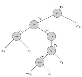
For ((x1 → x2) ∨ ¬((¬x1 ↔ x3) ∨ x4)) ∧ ¬x2, the tree is shown to the right and the expression resulting from the tree is shown below.
y1 ∧ (y1 ↔ (y2 ∧ ¬x2)) ∧ (y2 ↔ (y3 ∨ x4))
∧ (y3 ↔ (x1 → x2)) ∧ (y4 ↔ ¬y5)
∧ (y5 ↔ (y6 ∨ x4)) ∧ (y6 ↔ (¬x1 ↔ x3))
The remainder of the conversion uses DeMorgan's laws (see the text for the step by step description):
¬(a ∧ b) ≡ ¬a ∨ ¬b
¬(a ∨ b) ≡ ¬a ∧ ¬b
resulting in:
(¬y1 ∨ ¬y2 ∨ ¬x2) ∧ (¬y1 ∨ y2 ∨ ¬x2) ∧ (¬y1 ∨ y2 ∨ x2) ∧ (y1 ∨ ¬y2 ∨ x2).

A clique in an undirected graph G = (V, E) is a subset V' ⊆ V, each pair of which is connected by an edge in E (a complete subgraph of G). Examples of cliques of sizes between 2 and 7 are shown on the right.
The clique problem is the problem of finding a clique of maximum size in G. This can be converted to a decision problem by asking whether a clique of a given size k exists in the graph:
CLIQUE = {⟨G, k⟩ : G is a graph containing a clique of size k}
One can check a solution in polynomial time. How?

3-CNF-SAT is reduced to CLIQUE by a clever reduction illustrated in the figure. Given an arbitrary formula φ in 3-conjunctive normal form with k clauses, we construct a graph G and ask if it has a clique of size k as follows:
If there are k clauses in φ, we ask whether the graph has a k-clique. The claim is that such a clique exists in G if and only if there is a satisfying assignment for φ:
Any arbitrary instance of 3-CNF-SAT can be converted to an instance of CLIQUE in polynomial time with this particular structure. That means if we can solve CLIQUE we can solve any instance of 3-CNF-SAT, and since we know that 3-CNF-SAT is NPC, transitively, we can solve any instance in NP in polynomially related time. Be sure you understand why mapping an arbitrary instance of CLIQUE to a specialized instance of 3-CNF-SAT would not work.

A vertex cover of an undirected graph G = (V, E) is a subset V' ⊆ V such that if (u, v) ∈ E then u ∈ V' or v ∈ V' or both.
Each vertex "covers" its incident edges, and a vertex cover for G is a set of vertices that covers all the edges in E. For example, in the graph on the right, V' = {v, z} or V' = {v, w, y} are vertex covers. Note V' = V = {u, v, w, x, y, z} is also a vertex cover.
The Vertex Cover Problem asks to find a vertex cover of minimum size in G. Phrased as a decision problem,
VERTEX-COVER = {⟨G, k⟩ : graph G has a vertex cover of size k}
There is a straightforward reduction of CLIQUE to VERTEX-COVER, illustrated in the figure. Given an instance G=(V,E) of CLIQUE, one computes the complement of G, which we will call Gc = (V,Ē), where (u,v) ∈ Ē iff (u,v) ∉ E.

The graph G has a clique of size k iff the complement graph has a vertex cover of size |V| − k. (Note that this is an existence claim, not a minimization claim: a smaller cover may be possible.)
Intuition: none of the k vertices in the clique need to be in the cover.
Proof by contrapositive. We will prove the statement: "If there is no clique of size k in G, then there is no vertex cover of size |V| − k in Gc".
HAM-CYCLE = {⟨G⟩ : G contains a Hamiltonian cycle}
The Hamiltonian Cycle problem is shown to be in NPC by reduction of VERTEX-COVER to HAM-CYCLE.
Given graph G — an instance of VERTEX-COVER — the construction converts edges of G into subgraph "widgets" shown in the figure (a) below. The Hamiltonian Cycle will go through every vertex of the widget associated with edge each (u,v) if and only if one or both of the vertices of the edge (u,v) are in the covering set. There is one such widget for every edge (u,v) in G.

Any Hamiltonian cycle must include all the vertices in the widget (a), but there are only three ways to pass through each widget (b, c, and d in the figure). If only vertex u is included in the cover, we will use path (b); if only vertex v then path (d); otherwise path (c) to include both. (Not traversing the widget is not an option because at least one of the two vertices must be chosen to cover the edge.)
The widgets are then wired together in sequences that chain all the widgets that involve a given vertex, so if the vertex is selected all of the widgets corresponding to its edges will be reached.

Finally, k selector vertices are added, and wired such that each will select the kth vertex in the cover of size k. I leave it to you to examine the discussion in the text, to see how clever these reductions can be!
One of the more famous NPC problems is TSP: Suppose you are a traveling salesperson, and you want to visit n cities exactly once in a Hamiltonian cycle, but choosing a tour with minimum cost.
TSP = {⟨G, c, k⟩ : G = (V, E) is a complete graph,
c : V x V → ℕ,
k ∈ ℕ, and
G has a traveling-salesperson tour with cost at most k}
Only exponential solutions have been found to date, although it is easy to check a solution in polynomial time.
The reduction represents a HAM-CYCLE problem as a TSP problem on a complete graph, but with the cost of the edges in TSP being 0 if the edge is in the HAM-CYCLE problem, or 1 if not.
Many NP-Complete problems are of a numerical nature. We already mentioned integer linear programming. Another example is the subset-sum problem: given a finite set S of positive integers and an integer target t > 0, does there exist a subset of S that sums to t?
SUBSET-SUM = {⟨S, t : ∃ subset S' ⊆ S such that t = Σs∈S' s}
The proof reduces 3-CNF-SAT to SUBSET-SUM. Please see the text for the details of yet another clever reduction!
Briefly:

For example, see how this clause maps to the table shown:
(x1 ∨ ¬x2 ∨ ¬x3) ∧ (¬x1 ∨ ¬x2 ∨ ¬x3) ∧ (¬x1 ∨ ¬x2 ∨ x3) ∧ (x1 ∨ x2 ∨ x3).
One can find large catalogs of other problems online, starting with those identified in the book Garey & Johnson (1979), Computers and Intractability. See for example Wikipedia. Following Garey & Johnson's outline they list problems in:
There are also problems for which their status is as of yet unknown. Much work to do!
If you want to learn more about NP-completeness and how to come up with NP-completeness proofs yourself, various complexity classes, and the limits of what computers are able to compute, you should take ICS 441.