ICS 311 #12A: Dynamic Programming

Prerequisite Review

• ICS 141 (Linear Algebra)

Outline

1. Problem Solving Methods and Optimization Problems
2. Introducing DP with the Rod Cutting Example

Readings and Screencasts

• Read CLRS Sections 15.1-15.3. The focus is on the problem solving strategy: Read the examples primarily to understand the Dynamic Programming strategy rather than to memorize the specifics of each problem (although you might be asked to trace through some of the algorithms).
• Screencasts 12A, 12B (till minute 5:00), 12D (till minute 6:16) (also in Laulima)

Setting the Context

Problem Solving Methods

In this course we study many well defined algorithms, including (so far) those for ADTs, sorting and searching, and others to come to operate on graphs. Quality open source implementations exist: you often don't need to implement them.

But we also study problem solving methods that guide the design of algorithms for your specific problem. Quality open source implementations may not exist for your specific problem: you may need to:

• Understand and identify characteristics of your problem
• Match these characteristics to algorithmic design patterns.
• Use the chosen design patterns to design a custom algorithm.

Such problem solving methods include divide & conquer, dynamic programming, and greedy algorithms (among others to come).

Optimization Problems

An optimization problem requires finding a/the "best" of a set of alternatives (alternative approaches or solutions) under some quality metric (which we wish to maximize) or cost metric (which we wish to minimize).

Dynamic Programming is one of several methods we will examine. (Greedy algorithms and linear programming can also apply to optimization problems.)

Basic Idea of Dynamic Programming

Dynamic programming solves optimization problems by combining solutions to subproblems.

This sounds familiar: divide and conquer also combines solutions to subproblems, but applies when the subproblems are disjoint. For example, here is the recursion tree for merge sort on an array A[1..8]. Notice that the indices at each level do not overlap):

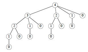
Dynamic programming applies when the subproblems overlap. For example, here is the recursion tree for a "rod cutting" problem to be discussed in the next section (numbers indicate lengths of rods). Notice that not only do lengths repeat, but also that there are entire subtrees repeating. It would be redundant to redo the computations in these subtrees.

Dynamic programming solves each subproblem just once, and saves its answer in a table, to avoid the recomputation. It uses additional memory to save computation time: an example of a time-memory tradeoff.

There are many examples of computations that require exponential time without dynamic programming but become polynomial with dynamic programming.

Example: Rod Cutting

This example nicely introduces key points about dynamic programming.

Suppose you get different prices for steel rods of different lengths. Your supplier provides long rods; you want to know how to cut the rods into pieces in order to maximize revenue. Each cut is free. Rod lengths are always an integral number of length units (let's say they are centimeters).

Input: A length n and a table of prices p_i for i = 1, 2, ..., n.

Output: The maximum revenue obtainable for rods whose lengths sum to n, computed as the sum of the prices for the individual rods.

We can choose to cut or not cut at each of the n-1 units of measurement. Therefore one can cut a rod in 2^n-1 ways.

If p_n is large enough, an optimal solution might require no cuts.

Example problem instance

Suppose we have a rod of length 4. There are 2^n-1 = 2³ = 8 ways to cut it up (the numbers show the price we get for each length, from the chart above):

Having enumerated all the solutions, we can see that for a rod of length 4 we get the most revenue by dividing it into two units of length 2 each: p₂ + p₂ = 5 + 5 = 10.

Optimal Substructure of Rod Cutting

Any optimal solution (other than the solution that makes no cuts) for a rod of length > 2 results in at least one subproblem: a piece of length > 1 remaining after the cut.

Claim: The optimal solution for the overall problem must include an optimal solution for this subproblem.

Proof: The proof is a "cut and paste" proof by contradiction: if the overall solution did not include an optimal solution for this problem, we could cut out the nonoptimal subproblem solution, paste in the optimal subproblem solution (which must have greater value), and thereby get a better overall solution, contradicting the assumption that the original cut was part of an optimal solution.

Therefore, rod cutting exhibits optimal substructure: The optimal solution to the original problem incorporates optimal solutions to the subproblems, which may be solved independently. This is a hallmark of problems amenable to dynamic programming. (Not all problems have this property.)

Continuing the example

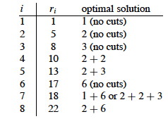
Here is a table of r_i, the maximum revenue for a rod of length i, for this problem instance.

To solve a problem of size 7, find the best solution for subproblems of size 7; 1 and 6; 2 and 5; or 3 and 4. Each of these subproblems also exhibits optimal substructue.

One of the optimal solutions makes a cut at 3cm, giving two subproblems of lengths 3cm and 4cm. We need to solve both optimally. The optimal solution for a 3cm rod is no cuts. As we saw above, the optimal solution for a 4cm rod involves cutting into 2 pieces, each of length 2cm. These subproblem optimal solutions are then used in the solution to the problem of a 7cm rod.

Quantifying the value of an optimal solution

The next thing we want to do is write a general expression for the value of an optimal solution that captures its recursive structure.

For any rod length n, we can determine the optimal revenues r_n by taking the maximum of:

• p_n: the price we get by not making a cut,
• r₁ + r_n-1: the maximum revenue from a rod of 1cm and a rod of n-1cm,
• r₂ + r_n-2: the maximum revenue from a rod of 2cm and a rod of n-2cm, ....
• r_n-1 + r₁

So, r_n = max (p_n, r₁ + r_n-1, r₂ + r_n-2, .... r_n-1 + r₁).

There is redundancy in this equation: if we have solved for r_i and r_n-i, we don't also have to solve for r_n-i and r_i.

A Simpler Decomposition

Rather than considering all ways to divide the rod in half, leaving two subproblems, consider all ways to cut off the first piece of length i, leaving only one subproblem of length n - i:

We don't know in advance what the first piece of length i should be, but we do know that one of them must be the optimal choice, so we try all of them.

Recursive Top-Down Solution

The above equation leads immediately to a direct recursive implementation (p is the price vector; n the problem size):

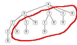
This works but is inefficient. It calls itself repeatedly on subproblems it has already solved (circled). Here is the recursion tree for n = 4:

In fact we can show that the growth is exponential. Let T(n) be the number of calls to Cut-Rod with the second parameter = n.

This has solution 2ⁿ. (Use the inductive hypothesis that it holds for j < n and then use formula A5 of Cormen et al. for an exponential series.)

Dynamic Programming Solutions

Dynamic programming arranges to solve each sub-problem just once by saving the solutions in a table. There are two approaches.

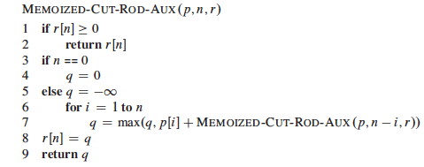
Top-down with memoization

Modify the recursive algorithm to store and look up results in a table r. Memoizing is remembering what we have computed previously.

The top-down approach has the advantages that it is easy to write given the recursive structure of the problem, and only those subproblems that are actually needed will be computed. It has the disadvantage of the overhead of recursion.

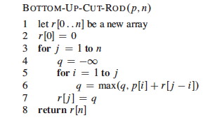
Bottom-up

One can also sort the subproblems by "size" (where size is defined according to which problems use which other ones as subproblems), and solve the smaller ones first.

The bottom-up approach requires extra thought to ensure we arrange to solve the subproblems before they are needed. (Here, the array reference r[j - i] ensures that we only reference subproblems smaller than j, the one we are currently working on.)

The bottom-up approach can be more efficient due to the iterative implementation (and with careful analysis, unnecessary subproblems can be excluded).

Asymptotic running time

Both the top-down and bottom-up versions run in Θ(n²) time.

• Bottom-up: there are doubly nested loops, and the number of iterations for the inner loop forms an arithmetic series.


• Top-down: Each subproblem is solved just once. Subproblems are solved for sizes 0, 1, ... n. To solve a subproblem of size n, the for loop iterates n times, so over all recursive calls the total number of iterations is an arithmetic series. (This uses aggregate analysis, covered in a later lecture.)

Constructing a Solution

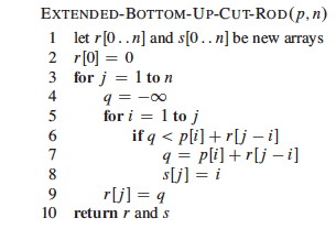
The above programs return the value of an optimal solution. To construct the solution itself, we need to record the choices that led to optimal solutions. Use a table s to record the place where the optimal cut was made (compare to Bottom-Up-Cut-Rod):

For our problem, the input data and the tables constructed are:

We then trace the choices made back through the table s with this procedure:

Trace the calls made by Print-Cut-Rod-Solution(p, 8)...

Four Steps of Problem Solving with Dynamic Programming

In general, we follow these steps when solving a problem with dynamic programming:

1. Characterize the structure of an optimal solution:
   • How are optimal solutions composed of optimal solutions to subproblems?
   • Assume you have an optimal solution and show how it must decompose
   • Sometimes it is useful to write a brute force solution, observe its redunancies, and characterize a more refined solution
   • e.g., our observation that a cut produces one to two smaller rods that can be solved optimally


2. Recursively define the value of an optimal solution:
   • Write a recursive cost function that reflects the above structure
   • e.g., the recurrence relation shown


3. Compute the value of an optimal solution:
   • Write code to compute the recursive values, memoizing or solving smaller problems first to avoid redundant computation
   • e.g., Bottom-Up-Cut-Rod


4. Construct an optimal solution from the computed information:
   • Augment the code as needed to record the structure of the solution
   • e.g., Extended-Bottom-Up-Cut-Rod and Print-Cut-Rod-Solution

The steps are illustrated in the next example.

Other Applications

Another application of Dynamic Programming is covered in the Cormen et al. textbook (Chapter 15.2). I briefly describe the problem here, but you are responsible for reading the details of the solution in the book.

Optimizing Matrix-Chain Multiplication

Many scientific and business applications involve multiplication of chains of matrices ⟨ A₁, A₂, A₃, ... A_n ⟩. Since matrix multiplication is associative, the matrices can be multiplied with their neighbors in this sequence in any order. The order chosen can have a huge difference in the number of multiplications required. For example suppose you have A, a 2x100 matrix, B (100x100) and C (100x20). To compute A*B*C:

(A*B) requires 2*100*100 = 20000 multiplications, and results in a 2x100 matrix. Then you need to multiply by C: 2*100*20 = 4000 multiplications, for a total of 24,000 multiplications (and a 2x20 result).

(B*C) requires 100x100x20 = 200000 multiplications, and results in a 100x20 matrix. Then you need to multiply by A: 2*100*20 = 4000 multiplications, for a total of 204,000 multiplications (and the same 2x20 result).

The Matrix-Chain Multiplication problem is to determine the optimal order of multiplications (not to actually do the multiplications). For three matrices I was able to figure out the best sequence by hand, but some problems in science, business and other areas involve many matrices, and the number of combinations to be checked grows exponentially.

Next

In Topic 12B, we will continue studying Dynamic Programming with more examples.